Sinuoidal Functions II
We will continue with sinusoidal type functions for the examples we will present, but now from . For the examples, we will use the following libraries,
# Libraries
import matplotlib.pyplot as plt
import numpy as np
import tensorflow as tf
and we're going to have to have is compact (closed and bounded).
Implementation in more dimensions, now for
Let The idea is to approximate a neural network to the continuous function , .
To calculate the points of the domain and the function in the domain,
# Omega domain
num_points = 256
omega_x = np.linspace(-2*np.pi, 2*np.pi, num_points, dtype="float64")
omega_y = np.linspace(-2*np.pi, 2*np.pi, num_points, dtype="float64")
omega_x, omega_y = np.meshgrid(omega_x, omega_y)
omega = np.stack([omega_x.ravel(), omega_y.ravel()], axis=1)
f_omega = np.sin(omega[:,0]+ omega[:,1]) # function sin(x+y) "implementation"

omega_x_tf = tf.convert_to_tensor(omega[:,0][:, np.newaxis])
omega_y_tf = tf.convert_to_tensor(omega[:,1][:, np.newaxis])
f_omega_tf = tf.convert_to_tensor(f_omega[:, np.newaxis])
construction of a neural network of
# Single hidden Layer Neural Network Phi wit M=400 hidden units
M = 400
weight_x = tf.Variable(tf.random.normal([1,M], dtype=tf.float64))
weight_y = tf.Variable(tf.random.normal([1,M], dtype=tf.float64))
beta = tf.Variable(tf.random.normal([M], dtype=tf.float64))
alpha = tf.Variable(tf.random.normal([M,1], dtype=tf.float64))

@tf.function
def Phi(x, y):
    return tf.matmul(
        tf.keras.activations.tanh(
            tf.add(
                tf.add(tf.matmul(x, weight_x), tf.matmul(y, weight_y)),
                beta
            )
        ),
        alpha
    )
training,
# training by gradient descent
learning_rate = 0.1
training_epochs = 4000

optimizer = tf.keras.optimizers.Adam(learning_rate)
mse = tf.keras.losses.MeanSquaredError()

for epoch in range(training_epochs):
    with tf.GradientTape() as tape:
        loss = mse(Phi(omega_x_tf, omega_y_tf), f_omega_tf)
    gradients = tape.gradient(loss, [weight_x, weight_y, beta, alpha])
    optimizer.apply_gradients(zip(gradients, [weight_x, weight_y, beta, alpha]))
For the visual element, we only plot the contours of the original function, the neural network and its absolute error,
# Graphic
f_omega = f_omega_tf.numpy().reshape((num_points, num_points))
f_omega_nn = Phi(omega_x_tf, omega_y_tf).numpy().reshape((num_points, num_points))

fig, axs = plt.subplots(1, 3, figsize=(18, 5))

cf1 = axs[0].contourf(omega_x, omega_y, f_omega, cmap='viridis')
axs[0].set_title("$\\sin(x^2+y^2)$")
plt.colorbar(cf1, ax=axs[0])

cf2 = axs[1].contourf(omega_x, omega_y, f_omega_nn, cmap='viridis')
axs[1].set_title("$\\Phi(x,y)$")
plt.colorbar(cf2, ax=axs[1])

cf3 = axs[2].contourf(omega_x, omega_y, np.abs(f_omega - f_omega_nn), cmap='inferno')
axs[2].set_title("$|\\sin(x^2+y^2) - \\Phi(x,y)|$")
plt.colorbar(cf3, ax=axs[2])

for ax in axs:
    ax.set_xlabel("$x$")
    ax.set_ylabel("$y$")

plt.tight_layout()
plt.show()
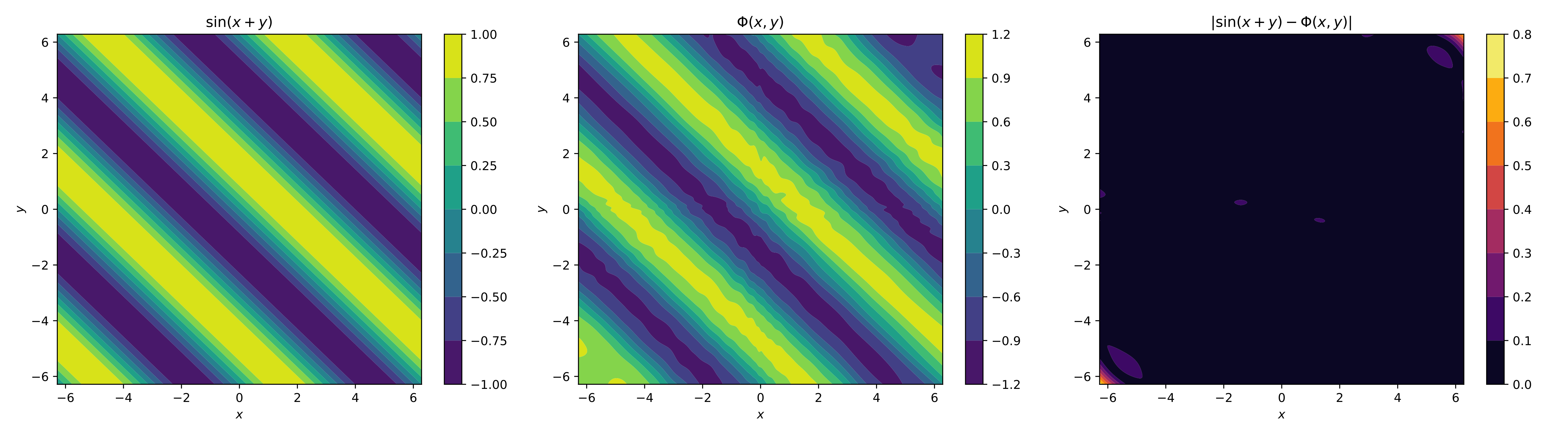
The image shows how the neural network approximated the function, and you can see they have the same nature. The approximation can be improved by adding more neurons and more epochs. There are also other options, such as applying training strategies and adding more layers. We'll briefly review all of this in the next section.
Another style of implementation, now for
As you can see, when we added a dimension, it became a bit more difficult to implement the functions, even though we only used a single layer. For this, there are equivalent ways to implement neural networks with multiple layers and outputs. In this case, a two-layer function with one output will be implemented.
Let The idea is to approximate a neural network to the continuous function , .
For this other type of implementation, we must use the following libraries,
from tensorflow.keras import models, layers
from tensorflow.keras.callbacks import ReduceLROnPlateau
from tensorflow.keras.optimizers import Adam
to calculate the points of the domain and the function in the domain,
num_points = 1024
omega_x = np.linspace(-2*np.pi, 2*np.pi, num_points, dtype="float64")
omega_y = np.linspace(-2*np.pi, 2*np.pi, num_points, dtype="float64")
omega_x, omega_y = np.meshgrid(omega_x, omega_y)
omega = np.stack([omega_x.ravel(), omega_y.ravel()], axis=1)
f_omega = np.sin(omega[:,0]**2+ omega[:,1]**2)
new construction of a neural network of ,
model = models.Sequential([
    layers.Input(shape=(2,)),
    layers.Dense(128, activation="tanh"),
    layers.Dense(128, activation="tanh"),
    layers.Dense(1)
])
this is less verbose and more compact, and it is easier to add layers as dimensions. Whenever possible, you should try to use this form, although there may be problems which would arise if you had to use the extended form.
New training settings,
model.compile(optimizer="adam", loss="mse")

reduce_lr = ReduceLROnPlateau(
    monitor='loss',       # or 'val_loss' if you have a validation set
    factor=0.5,           # reduces the learning rate by half
    patience=5,           # waits 5 epochs without improvement before reducing
    min_lr=1e-7,          # does not reduce the learning rate below this value
    verbose=1             # prints a message when the learning rate changes
)
as you can see, it's easier to configure the optimizer and the loss. It's also easier to add a strategy to reduce the learning rate.
Training,
model.fit(omega, f_omega, epochs=350, verbose=1, callbacks=[reduce_lr])
For the visual element, we only plot the contours of the original function, the neural network and its absolute error,
f_omega_tf = tf.convert_to_tensor(f_omega, dtype=tf.float64)
omega_x_tf = tf.convert_to_tensor(omega_x, dtype=tf.float64)
omega_y_tf = tf.convert_to_tensor(omega_y, dtype=tf.float64)

# Neural network evaluated
f_omega_nn = model.predict(omega).reshape((num_points, num_points))

# We restructure ground truth to graph
f_omega = f_omega.reshape((num_points, num_points))

fig, axs = plt.subplots(1, 3, figsize=(18, 5))

cf1 = axs[0].contourf(omega_x, omega_y, f_omega, cmap='viridis')
axs[0].set_title("$\\sin(x^2+y^2)$")
plt.colorbar(cf1, ax=axs[0])

cf2 = axs[1].contourf(omega_x, omega_y, f_omega_nn, cmap='viridis')
axs[1].set_title("$\\Phi(x, y)$")
plt.colorbar(cf2, ax=axs[1])

cf3 = axs[2].contourf(omega_x, omega_y, np.abs(f_omega - f_omega_nn), cmap='inferno')
axs[2].set_title("$|\\sin(x^2+y^2) - \\Phi|$")
plt.colorbar(cf3, ax=axs[2])

for ax in axs:
    ax.set_xlabel("$x$")
    ax.set_ylabel("$y$")

plt.tight_layout()
plt.show()
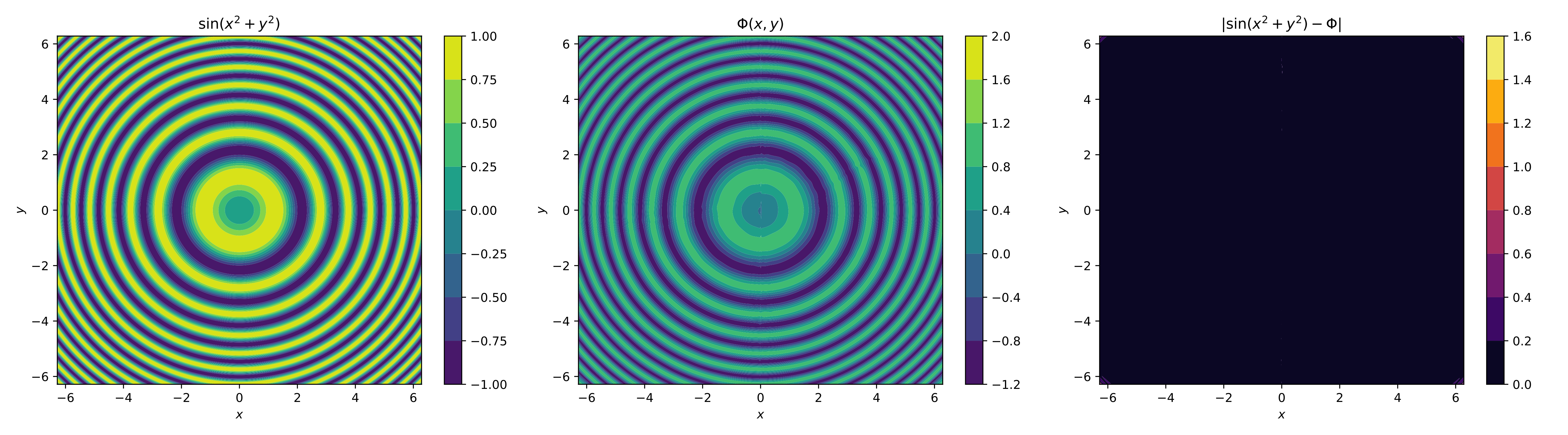
It can be noted that with the changes, the neural network better approximated the function, considering its more difficult nature to reach. In fact, it's a very good approximation; the difficulty lies in the corners, but these can be improved with more neurons, perhaps another layer, and more epochs.