Sinuoidal Functions II
We will continue with sinusoidal type functions for the examples we will present, but now from . For the examples, we will use the following libraries,
# Libraries
import matplotlib.pyplot as plt
import numpy as np
import tensorflow as tf
and we're going to have to have is compact (closed and bounded).
Implementation in more dimensions, now for
Let The idea is to approximate a neural network to the continuous function , .
To calculate the points of the domain and the function in the domain,
# Omega domain
num_points = 256
omega_x = np.linspace(-2*np.pi, 2*np.pi, num_points, dtype="float64")
omega_y = np.linspace(-2*np.pi, 2*np.pi, num_points, dtype="float64")
omega_x, omega_y = np.meshgrid(omega_x, omega_y)
omega = np.stack([omega_x.ravel(), omega_y.ravel()], axis=1)
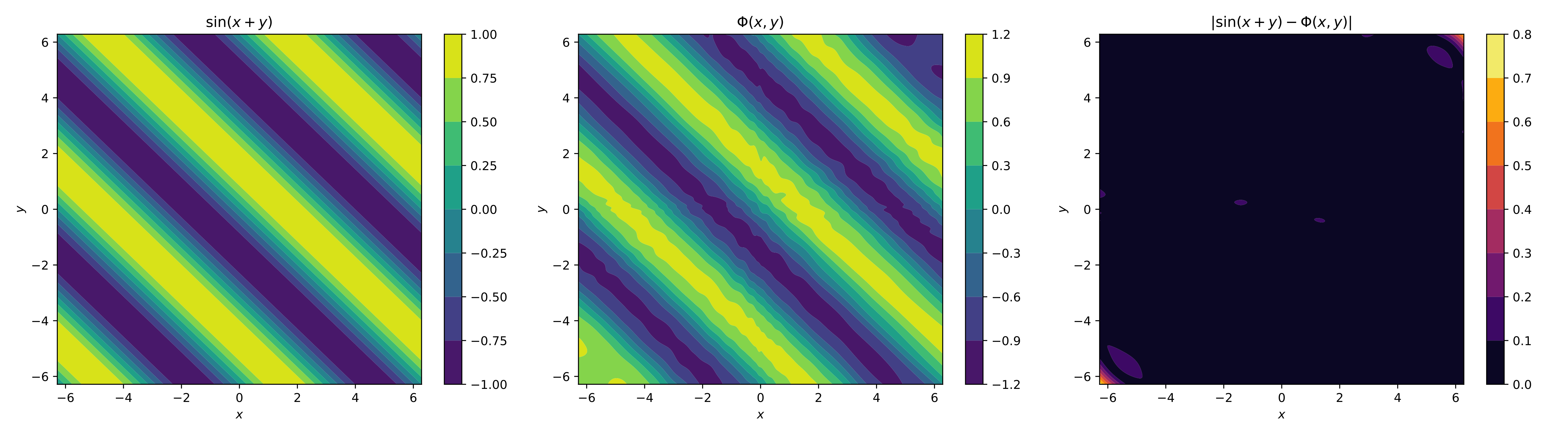
f_omega = np.sin(omega[:,0]+ omega[:,1]) # function sin(x+y) "implementation"
omega_x_tf = tf.convert_to_tensor(omega[:,0][:, np.newaxis])
omega_y_tf = tf.convert_to_tensor(omega[:,1][:, np.newaxis])
f_omega_tf = tf.convert_to_tensor(f_omega[:, np.newaxis])
Construction of a neural network of
# Single hidden Layer Neural Network Phi wit M=400 hidden units
M = 400
weight_x = tf.Variable(tf.random.normal([1,M], dtype=tf.float64))
weight_y = tf.Variable(tf.random.normal([1,M], dtype=tf.float64))
beta = tf.Variable(tf.random.normal([M], dtype=tf.float64))
alpha = tf.Variable(tf.random.normal([M,1], dtype=tf.float64))

@tf.function
def Phi(x, y):
    return tf.matmul(
        tf.keras.activations.tanh(
            tf.add(
                tf.add(tf.matmul(x, weight_x), tf.matmul(y, weight_y)),
                beta
            )
        ),
        alpha
    )
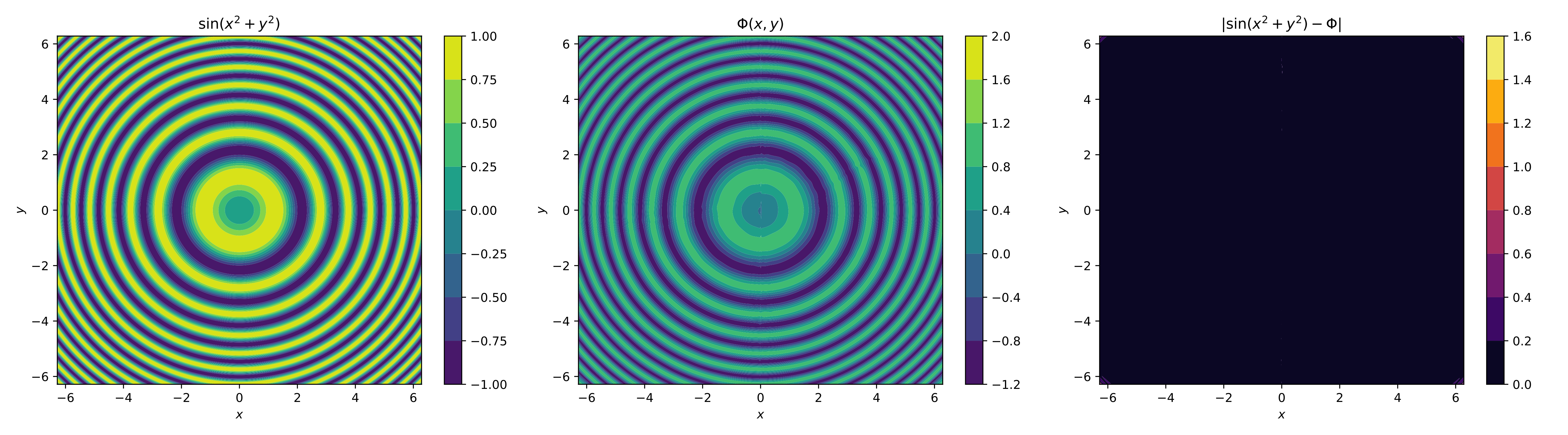
For the visual element, we only plot the contours of the original function, the neural network and its absolute error,
# training by gradient descent
learning_rate = 0.1
training_epochs = 4000

optimizer = tf.keras.optimizers.Adam(learning_rate)
mse = tf.keras.losses.MeanSquaredError()

for epoch in range(training_epochs):
    with tf.GradientTape() as tape:
        loss = mse(Phi(omega_x_tf, omega_y_tf), f_omega_tf)
    gradients = tape.gradient(loss, [weight_x, weight_y, beta, alpha])
    optimizer.apply_gradients(zip(gradients, [weight_x, weight_y, beta, alpha]))
For the visual, we only plot the contours of the original function, the neural network, and the absolute error,
# Graphic
f_omega = f_omega_tf.numpy().reshape((num_points, num_points))
f_omega_nn = Phi(omega_x_tf, omega_y_tf).numpy().reshape((num_points, num_points))

fig, axs = plt.subplots(1, 3, figsize=(18, 5))

cf1 = axs[0].contourf(omega_x, omega_y, f_omega, cmap='viridis')
axs[0].set_title("$\\sin(x^2+y^2)$")
plt.colorbar(cf1, ax=axs[0])

cf2 = axs[1].contourf(omega_x, omega_y, f_omega_nn, cmap='viridis')
axs[1].set_title("$\\Phi(x,y)$")
plt.colorbar(cf2, ax=axs[1])

cf3 = axs[2].contourf(omega_x, omega_y, np.abs(f_omega - f_omega_nn), cmap='inferno')
axs[2].set_title("$|\\sin(x^2+y^2) - \\Phi(x,y)|$")
plt.colorbar(cf3, ax=axs[2])

for ax in axs:
    ax.set_xlabel("$x$")
    ax.set_ylabel("$y$")

plt.tight_layout()
plt.show()
Another style of implementation, now for
As you can see, when we added a dimension, it became a bit more difficult to implement the functions, even though we only used a single layer. For this, there are equivalent ways to implement neural networks with multiple layers and outputs.